UnaXL Excel Add-in — Training Guide

Environment: Windows & Mac Office Excel

Overview

UnaXL is an Excel add-in that connects to data models and lets you configure dynamic grids that pull live data directly into your spreadsheets. Once set up, grids refresh with the latest data whenever you click Refresh Data, picking up any filter selections, added members, or query changes you have made — all without leaving Excel. You can also edit values in a grid and save them back to Una.

This guide walks through every feature of the add-in from first launch through to advanced grid management.

Getting Started

Launching the Add-in

With the UnaXL add-in sideloaded, open Microsoft Excel and locate the UnaXL tab in the Ribbon. Click Show Task Pane to open the UnaXL task pane on the right side of the screen.

tip

If a workbook has been published to Una with Open UnaXL with this workbook turned on, the task pane opens automatically whenever that workbook is opened. See Workbook Settings.

Logging In

UnaXL supports two single sign-on providers. Choose whichever matches the account your organisation uses:

• Microsoft — Click Microsoft in the task pane. A Microsoft authentication popup appears listing your available accounts. Select an account and complete the sign-in flow. Once authenticated, you are redirected to the UnaXL dashboard.
• Google — Click Google in the task pane. A Google authentication popup appears listing your available accounts. Select an account and complete the sign-in flow. Once authenticated, you are redirected to the UnaXL dashboard.

Both providers follow the same flow: a provider popup, account selection, sign-in, and redirect to the dashboard. You only need to sign in with one provider — use the same one each session for a consistent experience.

If your account has access to more than one tenant, a welcome screen appears after sign-in showing your account. Choose a workspace from the Select Tenant list and click Sign In to continue to the dashboard.

The Dashboard

After login, the task pane shows a header bar and two tabs.

The header bar contains:

• Tenant badge — the name of the tenant you are currently working in
• Workbook settings (gear icon) — repository and workbook-wide behaviour, see Workbook Settings
• Profile (your initials) — your account details, tenant switching, and sign out

Below the header:

• Data Tab — refresh and save data, open line item details, and pick filter values
• Mapping Tab — configure grids, filters, triggers, variables, block formatting, and worksheet protection

The Data tab has three buttons:

• Refresh Data — fetch the latest data from Una into every grid in the workbook
• Save Data — send edited grid values on the active sheet back to Una
• Line Item Details — view or edit the line items behind a selected data cell, see Line Item Details

The UnaXL Ribbon

The UnaXL Ribbon tab groups the add-in's commands:

Group	Button	What it does
UnaXL	Show Task Pane	Opens the UnaXL task pane
Data	Get Data	Same as Refresh Data in the task pane
Data	Send Data	Same as Save Data in the task pane
Visibility	Hide Cells / Show Cells	Hide or show marked rows and columns, see Hiding and Showing Rows and Columns
Row / Column	Add Row / Add Column	Append a member to the selected grid, see Allow Add Row / Add Column

The Ribbon buttons are enabled only once you are signed in and a tenant is selected. Get Data and Send Data also need at least one grid in the workbook, and Add Row / Add Column need a cell inside a grid to be selected. Running Get Data or Send Data from the Ribbon opens the task pane so you can follow the progress.

Switching Tenant

If you have access to more than one tenant, click the Profile icon and choose a different tenant from the Select Tenant dropdown. The add-in reloads models, grids, and filters for the new tenant and confirms the switch with a notification.

Signing Out

Click the Profile icon (your initials) in the top-right corner of the task pane. The profile popup displays your name and email address, and — if you have access to more than one tenant — the tenant selector. Click Sign Out to log out and return to the login screen.

In some environments the profile popup also shows Privacy settings, where you can choose whether to allow privacy-protected session replay that helps the UnaXL team diagnose stability problems. Form entries and images are always masked.

Opening Older Workbooks

When you open a workbook created with an earlier version of UnaXL, the add-in may update its stored grids and filters to the current format. A notification tells you when this starts and how many grids and filter sets were updated.

If the workbook contains data for more than one tenant, a Choose which data to keep dialog appears. Select the tenant whose grids and filters should be kept. The other tenants' data no longer appears in the add-in, but a copy is kept in a hidden backup inside the workbook.

Grids

Grids are the foundation of UnaXL. A grid is a structured data table written into your Excel worksheet, driven by a query you configure. The add-in tracks each grid using named ranges and refreshes it whenever you click Refresh Data or change its configuration.

Creating a Grid

1. Navigate to the Mapping tab and click New Grid. The grid Settings popup opens.
2. Give the grid a Name.
3. On the Queries tab, click Edit Query to open the Model Query Editor. Here you define what data the grid will display:
   • Select a Model, a Data Type, and optionally a Time perspective
   • Add Filters to narrow the result set
   • Add Row and Column hierarchies to shape the table structure
   • Optionally add Data Filters — only members matching these filters contribute data, and parents are rolled up from the matching members only
   • Turn on Use dimension roles to build the query from dimension roles instead of specific dimensions
4. Click OK to close the Query Editor and return to the grid Settings.
5. Optionally adjust options on the Configuration tab (see Configuration Options), then click OK.

The add-in fetches data from the configured source and inserts it into the Excel worksheet as a structured table with labelled rows, columns, and headers.

Named Ranges

Each grid automatically creates three independent named ranges in Excel:

• Data Range — covers the data cells of the grid
• Column Header Range — covers the column header row
• Row Header Range — covers the row header column

These named ranges are standard Excel named ranges and can be referenced and manipulated directly within Excel. This makes them available for a wide range of use cases — such as driving charts and pivot tables, referencing grid data in formulas elsewhere in the workbook, applying conditional formatting across a grid region, or integrating UnaXL data with other Excel-based workflows. The named ranges update automatically when the grid refreshes, so any downstream references always reflect the latest data.

In the Mapping tab, each grid under Grids on this sheet shows a chip for each of its ranges — CH (column headers), RH (row headers), and Data. Click a chip to select that range in the worksheet. Grids with additional query ranges show numbered chips (CH0, CH1, and so on).

Editing a Grid

In the Mapping tab, click the Edit Grid (Pencil) icon beside the grid name. The grid Settings popup opens with all current configuration loaded. Click Edit Query to modify Filters, Rows, Columns, or Members. Click OK through both popups when done — the grid refreshes automatically and replaces the existing data with the updated result.

Deleting a Grid

Click the Delete Grid (Trash) icon beside a grid in the Mapping tab. A confirmation appears — click Delete to proceed. The grid and its cell contents are removed from the worksheet, and all associated named ranges are cleared. This cannot be undone.

Refreshing Grid Data

Click Refresh Data in the Data tab (or Get Data in the Ribbon) to fetch the latest data for every grid in the workbook. Grids on the active sheet are refreshed first, followed by grids on the other sheets. When the refresh finishes, a summary notification shows how many grids loaded successfully and lists any grid that failed, with the reason.

Changing a filter does not refresh grids on its own — this lets you set several filters first and then fetch the data once. Click Refresh Data after you have made your selections.

Saving Data Back to Una

Edit values in a grid's data cells, then click Save Data in the Data tab (or Send Data in the Ribbon). The values from every grid on the active sheet that has Allow Save turned on are sent back to Una, and a notification confirms whether the save succeeded.

Save Data stops with an explanatory message when:

• There is no grid on the active sheet
• No grid on the sheet has Allow Save enabled
• A grid contains subtotal rows, or rows or columns inserted by a block format rule — turn those off and refresh before saving
• A filter's current value is not a member of that filter — pick a valid value and try again
• The action column is on but no rows are marked update

After a successful save, any triggers configured in the workbook run, and — if Refresh on save is on — every grid in the workbook is refreshed.

Cell Details

Click Cell Details in the Mapping tab, then select a cell inside a grid. The Cell Metadata panel shows the members that make up that cell, grouped into Columns and Rows, with each dimension's position number. Use the Key, Name, and Caption buttons to choose which member details are shown. Click the close icon, or Cell Details again, to hide the panel.

Filters

Filters let you control which dimension members appear in a grid, and expose those selections as interactive dropdowns directly in your Excel cells.

Filter Sets

A filter set is a named collection of one or more filters. Filter sets are numbered in the order they were created — the first set is index 0, the next is index 1, and so on. The first set always exists and cannot be deleted.

A grid's query responds to a filter selection through a parameter variable built from the filter's dimension and its filter set's index:

• {Parameter.period.0.Key} — the Period filter in the first filter set
• {Parameter.period.1.Key} — the Period filter in the second filter set
• {Parameter.period.2.Key} — the Period filter in the third filter set, and so on

The number in the middle of the variable is the filter set's index. If you only need one Period selection, put the Period filter in the first set and reference it as index 0. If you need a second, independent Period selection — for example, to compare two periods side by side — add a Period filter to a second filter set and reference it as index 1. Within a single filter set, each filter is identified by its own dimension, so one set can hold a Period filter and an Account filter at the same time, referenced as {Parameter.period.0.Key} and {Parameter.account.0.Key}.

Besides .Key, each filter also provides .Name and .Caption (and the plural forms .Keys, .Names, and .Captions), so a query can use whichever member property it needs.

Creating a Filter

1. In the Mapping tab, scroll to the Filter Sets section.
2. To add filters to an existing set, click the Edit Filter Set (Pencil) icon on that set. To start a new set, click Add Filter Set (+).
3. The Edit Filter Set popup opens. Move dimensions from Available Dimensions into Selected Filters.
4. Optionally select a filter under Selected Filters to configure it — for example, a default value (None, Value, SQL Query, or Dimension Query). Use Advanced for more configuration options; switching a filter to advanced mode is permanent.
5. Close the popup to save. The filter set's configuration is stored in the add-in's hidden sheet.

Use the Delete Filter (Trash) icon to remove a single filter, or Delete Filter Set to remove a whole set (except the first one). Both ask for confirmation.

Dimension Filters and Dimension-Role Filters

The Use dimension role switch at the top of the Filter Sets section chooses whether filters are built from specific dimensions or from dimension roles. The two kinds are stored differently, so switching modes removes all existing filters — a confirmation (Switch and clear) appears first. Dimension-role filters also need a filter scope, set in Workbook Settings.

Filters in Excel

Once created, a filter appears in the Data tab under its filter set's name. Click it to open a searchable, hierarchical tree of members and pick a value. Date filters show a date picker instead. Click the × beside a selected value to reset the filter to its default.

When a filter is placed in a worksheet cell (see below), that cell shows a dropdown list of the filter's members, so users can pick values directly from the spreadsheet — no need to open the task pane. If a value typed into the cell is not a member of the filter, the selection is rejected and a notification explains why.

Placing a Filter with the Filter Picker

1. In Excel, select the cell where the filter should appear.
2. In the Mapping tab, click the filter's Pick cell for filter icon.

The filter dropdown is placed in the selected cell, and the filter shows Bound to cell in the Mapping tab. To remove the placement, click the same icon again (its tooltip now reads Remove cell binding). A cell can hold only one filter — if the selected cell is already used by another filter, you are asked to pick a different cell.

Multiple Filters on One Sheet

You can create as many filter sets as needed on a single worksheet. Each filter is independently assigned to its own Excel cell and displayed separately in the Filter Sets section.

Linking a Filter Set to a Grid

To make a grid respond dynamically to a filter selection:

1. Open the grid in Edit mode and click Edit Query.
2. In the Filters section, remove the existing member and click + to open the Add Member popup.
3. Set a By value, then select a Key variable. The variable references the filter's dimension and its filter set's index — for example, {Parameter.period.0.Key} refers to the Period filter in the first filter set.
4. Choose a Relationship (Self, Descendants, Children, etc.) to define how the selected member's hierarchy is applied to the query.
5. Click Accept, then OK through both popups.

From this point on, after you change the filter value, click Refresh Data and the grid shows data for the newly selected member.

tip

To drive a grid with multiple filters simultaneously, repeat this process for each dimension you want to make dynamic, referencing the appropriate filter set index for each — 0 for filters in the first set, 1 for the second, and so on.

Configuration Options

Each grid has a Configuration tab within its Settings popup, offering additional controls that go beyond the basic query setup.

Allow Retrieve and Allow Save

• Allow Retrieve — when on, Refresh Data writes values into the grid's data cells. Turn it off to keep your own formulas in the data block while still refreshing headers.
• Allow Save — when on, the grid's values are sent to Una by Save Data. Grids without Allow Save are skipped.

Allow Save is switched off automatically while subtotals or block format rules that insert rows or columns are enabled, because those cells do not map to data members.

Multiple Row and Column Headers

A grid can display more than one header property per row or column — for example, showing Name, Caption, and Key simultaneously.

In the Configuration tab, use the Column Headers and Row Headers dropdowns to select a property, then click + to add it. Repeat for each additional property. Click OK — the grid refreshes and the additional headers appear alongside the existing data.

Choose the Custom property to build a header from a formula. Type an opening brace ({) in the Custom formula box to see suggestions for row or column metadata, such as a member's name, caption, key, or level.

Headers as Text

When Headers as Text is on, header values are written as text, so Excel does not reinterpret keys or names that look like numbers or dates.

Fill Missing Values

When a query returns empty or null cells, enabling this option automatically substitutes 0 in their place.

Enable the Fill Missing Values checkbox in the Configuration tab and click OK. On the next refresh, all empty cells display 0. Cells that already contain data are unaffected.

Exclude from Grid

Under Exclude from Grid, tick Without Column Headers, Without Row Headers, or Without Data to leave that block out of the grid entirely. An excluded block is not written and gets no named range, and the remaining blocks move up or left to take its place.

note

Excluding the data block leaves the grid with headers only, so it can no longer save values back. To keep the data block but preserve your own formulas in it, turn off Allow Retrieve instead.

Grid Resizing

Resizing controls how a grid grows and shrinks when a refresh returns more or fewer rows or columns. Choose one of two modes:

• Local Resizing — tick Row and/or Column. The grid adds or removes cells below it (rows) or to its right (columns), shifting only the neighbouring cells.
• Global Resizing — tick Insert Row, Delete Row, Insert Column, and/or Delete Column. The grid inserts or deletes entire worksheet rows and columns as the data grows or shrinks. With none ticked, the grid is populated in place.

caution

Both modes can affect other content on the worksheet. Local resizing may move nearby grids, and global resizing shifts every cell on the sheet — not just this grid. Use these options with care.

Hide Empty Rows

When Hide Empty Rows is on and the query returns no data, the grid's rows are hidden instead of being left blank. They are shown again as soon as the grid returns data. Excel hides entire worksheet rows, so any other grid sharing those rows is hidden too.

Dynamic Grid

Dynamic Grid keeps the grid's named ranges aligned with its top-left corner cell. If the grid is moved manually, the named ranges are restored to their original positions on the next refresh.

Allow Add Row / Add Column

Enabling Allow Add Row/Column in the Configuration tab activates dedicated Ribbon buttons that let you append new members to the grid without reconfiguring the full query.

Once enabled, return to the Excel worksheet and open the UnaXL Ribbon tab. Select a cell inside the grid, then:

• Click Add Row → choose a member from the row hierarchy popup → click Confirm
• Click Add Column → choose a member from the column hierarchy popup → click Confirm

The grid refreshes with the new member added. Existing rows and columns are unaffected.

Hiding and Showing Rows and Columns

You can suppress rows or columns from view without removing their data or altering the grid configuration.

• To hide a row: Type HideRow into any cell in the target row.
• To hide a column: Type HideColumn into any cell in the target column.
• Click Hide Cells in the UnaXL Ribbon. Every marked row and column on the active sheet is hidden — you do not need to select the marked cells first.
• To restore hidden content: Click Show Cells in the Ribbon. All marked rows and columns on the active sheet reappear with their original data intact.

The markers are not case-sensitive.

Additional Query Ranges

A single grid can draw from more than one query range, letting you append supplementary periods or measures alongside the primary dataset.

1. Open the grid's Query Editor.
2. In the Row/Column range selector, click + to create a new range at index 1.
3. Configure the Rows and/or Columns for this range. Add further ranges if needed.
4. Click OK through both popups.

The grid refreshes and the additional data is appended to the existing table. Data from the original range (index 0) is preserved in full.

Subtotals

UnaXL can insert subtotal lines into a grid and group them with Excel's outline controls. There are two ways to set this up on the Configuration tab.

Subtotal rules (recommended):

1. Under Subtotal, tick Enable subtotal rules and click Add Subtotal Rule.
2. Choose the Axis (Rows or Columns) and the dimensions to Break on. A subtotal line is inserted wherever the member of a break-on dimension changes.
3. Optionally choose a Block Format to style the subtotal line (see Block Formatting), with Apply content and Apply style to control what the template contributes. Leave it on Default subtotal line to use the built-in style.
4. Tick Grouping to group the detail lines under each subtotal with Excel's outline controls.

Condition-based subtotal and Excel grouping:

1. Tick Enable subtotal and Excel grouping.
2. Enter a Grouping condition — a row metadata field such as meta.row.level or meta.row.caption. Consecutive rows with the same value form a group. Type meta.row. or an opening brace to see suggestions.
3. Choose a Subtotal placement: Insert Above, Insert After, or Overwrite Next Row (keeps the next row's header and replaces its data with SUBTOTAL formulas).

Enabling condition-based subtotals also turns on dynamic grid and row resizing. To remove subtotals, turn them off and click Refresh Data — the subtotal rows and groups are removed and the source values restored.

note

A grid with subtotal rows cannot be saved back to Una. Turn subtotals off and refresh before using Save Data.

Formatting

UnaXL grids behave like ordinary Excel ranges when it comes to cell formatting. Number formats, fonts, fills, borders, and alignment are applied exactly as they would be anywhere else in the workbook, and they are preserved across refreshes. For repeatable, rule-driven styling, UnaXL also offers Block Formatting.

How Formatting Carries Over to New Cells

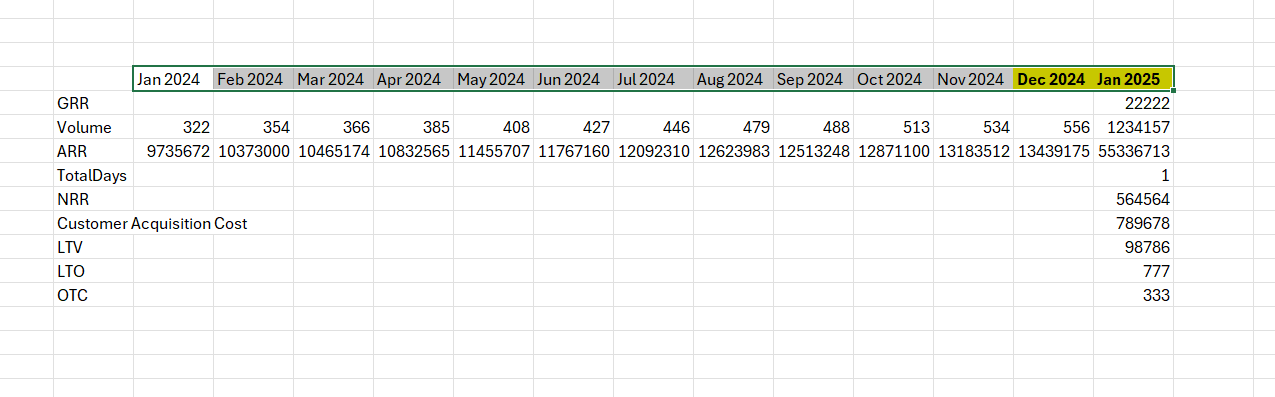
When a grid grows — because a refresh returns additional periods, or because you add a row or column — UnaXL applies the formatting of the last existing cell in that direction to the newly created cells. This mirrors standard Excel fill behaviour: the most recent cell in a header row or data column acts as the template for whatever is added next.

The principle applies uniformly to every part of the grid. A new header cell takes on the styling of the header that immediately precedes it — fill, font, and borders included — so the visual identity of the header band extends naturally as the grid widens or lengthens. Likewise, a new data cell adopts the styling of the data cell that came before it in the same direction, carrying forward number formats, decimal places, currency symbols, and conditional formatting. Because each new cell is shaped by its nearest existing neighbour rather than by a fixed default, the grid stays internally consistent without any manual intervention.

In the example below, the highlighted Dec 2024 and Jan 2025 header cells illustrate this: their fill, font, and border styling propagated automatically from the header cells that preceded them.

Because of this, the recommended workflow is to format the grid once — set your number formats, header styling, and column widths the way you want them — and let UnaXL propagate that formatting automatically as the grid expands. You do not need to reformat after every refresh.

Formatting from the First Cell

Two options on the grid's Configuration tab apply one cell's formatting to a whole column or row of data on every refresh. Only one can be on at a time:

• Format based on first column cell — each data column takes its formatting from its first (top) data cell.
• Format based on first row cell — each data row takes its formatting from its first (left-most) data cell.

Format the first cell the way you want, and the rest of that column or row follows it.

Manual Formatting

You are free to apply any standard Excel formatting to a grid at any time:

• Number formats (currency, percentage, thousands separators, decimal places)
• Fonts, colours, fills, and borders
• Conditional formatting across the grid region (the Named Ranges make this straightforward to target)
• Column widths and row heights

These are retained when the grid refreshes. Only the cell values are replaced on refresh; the formatting you applied stays in place and continues to propagate to any new cells.

Block Formatting

Block formatting lets you design a formatted template once and have UnaXL apply it to matching rows or columns of a grid on every refresh — for example, to highlight total lines or insert a spacer row after each group.

Creating a block format:

1. Format a range of cells in the worksheet the way the template should look, including any values or formulas it should carry.
2. In the Mapping tab, under Block Formatting, click Add Block Formatting.
3. Enter a Name (letters, numbers, and underscores only).
4. Select the template cells in the sheet and click the crosshair (Use current selection), or type the Range (for example, Sheet1!A1:D10).
5. Choose the Direction: Row for a template that runs along a row, or Column for one that runs down a column.

The block format is stored as a workbook named range. Click a block format in the list to select its range, use Edit Block Formatting to change it, or Delete Block Formatting to remove the named range (cell contents are not changed). The Block Formatting settings icon offers Extend to the grid edge, which repeats the template's last cell to the edge of the grid.

Applying block formats to a grid:

1. Open the grid's Settings and go to the Configuration tab.
2. Under Block Format, tick Enable block format and click Add Block Format Rule.
3. Enter a Condition that decides which rows or columns the rule applies to. Use TRUE for a rule that always applies.
4. Choose the Block Format to apply, an Anchor (None, Row, or Column), and a Mode:
   • Overwrite — formats the matching cells in place
   • Insert Before / Insert After — inserts whole worksheet rows or columns next to each match. These need an anchor: Column inserts rows, Row inserts columns. Inserted lines are removed and re-inserted on every refresh.
5. Choose whether to Apply content, Apply style, or both, and whether to Allow overlap with other rules.
6. Under Advanced, choose a Paste special option — All, Formulas, Values, or Formats — and optionally Skip blanks.

note

While a rule inserts rows or columns, Allow Save is turned off for that grid. Change those rules to Overwrite (or turn them off) and refresh before saving data.

Formulas

UnaXL grids live in ordinary Excel cells, so you can reference grid data in formulas exactly as you would any other range. Every standard Excel function — SUM, AVERAGE, VLOOKUP, INDEX, MATCH, and the rest — works against grid cells with no special syntax.

Using Named Ranges in Formulas

The most powerful way to reference grid data is through the named ranges UnaXL creates automatically for every grid (Data Range, Column Header Range, and Row Header Range). Because these are standard Excel named ranges, you can use them directly in formulas anywhere in the workbook, and they update automatically whenever the grid refreshes — so your formulas always reference the latest data.

You can also create your own named ranges over grid values and reference those.

Ways to Reference a Cell in a Named Range

The following patterns all reference cells within a named range. For these examples, assume the grid's Data Range named range UNA_New_Matrix_Data_R0_C0 = A1:A10.

1. Direct named range

=UNA_New_Matrix_Data_R0_C0

2. INDEX

=INDEX(UNA_New_Matrix_Data_R0_C0,1)    → first cell
=INDEX(UNA_New_Matrix_Data_R0_C0,5)    → fifth cell

3. OFFSET

=OFFSET(UNA_New_Matrix_Data_R0_C0,4,0)

4. Using ROW position

=INDEX(UNA_New_Matrix_Data_R0_C0,ROW(A1))

5. MATCH / XMATCH + INDEX

=INDEX(UNA_New_Matrix_Data_R0_C0,MATCH("Jan",Months,0))
=INDEX(UNA_New_Matrix_Data_R0_C0,XMATCH("Jan",Months))

6. Dynamic array functions

=TAKE(UNA_New_Matrix_Data_R0_C0,1)
=DROP(UNA_New_Matrix_Data_R0_C0,1)
=CHOOSECOLS(UNA_New_Matrix_Data_R0_C0,2)
=CHOOSEROWS(UNA_New_Matrix_Data_R0_C0,3)

7. Implicit intersection

=@UNA_New_Matrix_Data_R0_C0

8. First or last cell

=INDEX(UNA_New_Matrix_Data_R0_C0,1)                              → first cell
=INDEX(UNA_New_Matrix_Data_R0_C0,ROWS(UNA_New_Matrix_Data_R0_C0))   → last cell

9. Address-based reference

=INDIRECT("UNA_New_Matrix_Data_R0_C0")
=ADDRESS(ROW(INDEX(UNA_New_Matrix_Data_R0_C0,3)),COLUMN(INDEX(UNA_New_Matrix_Data_R0_C0,3)))

10. Spill range reference

=UNA_New_Matrix_Data_R0_C0#

Referencing Filter Selections

When a filter is placed in a cell, UnaXL also creates workbook names for its current selection, using the same pattern as the query variables: Parameter.<dimension>.<filter set index>.Key, .Name, and .Caption. You can use these in formulas — for example, in a report title:

="Actuals for "&Parameter.period.0.Caption

FP&A Examples

Assume two named ranges: Actuals = B2:M2 and Budget = B3:M3.

=INDEX(Actuals,MONTH(TODAY()))      → current month's actual
=INDEX(Actuals,MONTH(TODAY())-1)    → prior month's actual
=INDEX(Actuals,5)-INDEX(Budget,5)   → May variance (actual − budget)

tip

INDEX(named_range, row, column) is typically the most reliable way to reference a cell within a named range. It is unambiguous, works consistently across Excel versions, and does not break when the range is moved or resized.

Variables

Variables let a grid's query use values that come from somewhere other than a filter — a SQL or dimension query, or a cell in the workbook. Both kinds are managed in the Mapping tab and can be referenced in queries as {Variable.<name>.Key}.

Dashboard Variables

A dashboard variable takes its value from a query that runs against Una.

1. In the Mapping tab, under Dashboard Variables, click Add Dashboard Variable (+).
2. Enter a Name and, optionally, a Description.
3. Choose the Type:
   • SQL Query — write the query in the SQL editor
   • Dimension Query — click Edit Query to select members
4. Click Save.

A dashboard variable's query can itself reference filter selections (for example, {Parameter.period.0.Key}). Such variables are re-evaluated whenever the filter changes and before every refresh. Use the Pencil and Trash icons to edit or delete a variable.

Form Variables

A form variable sends the value of an Excel named range with every query, so users can type an input into a cell and have grids respond to it.

1. In Excel, define a named range of a few cells or a named formula (Formulas > Name Manager).
2. In the Mapping tab, under Form Variables, click Add Form Variable (+) and pick the named range from the list.

The variable is listed with its query token, for example {Variable.TargetMargin.Key}. Named ranges on hidden worksheets are marked with an icon, and a name already used by a dashboard variable cannot be added. Removing a form variable stops it being sent with queries; the named range itself stays in the workbook.

Triggers

Triggers are SQL statements that run in Una immediately after a successful Save Data — for example, to recalculate dependent figures or log the save.

1. In the Mapping tab, under Triggers, click Add Trigger (+).
2. In the New SQL Trigger popup, enter a Name, an optional Description, and the SQL Query.
3. Click Save.

Every trigger in the workbook runs after all grids on the sheet have saved successfully. A notification reports how many SQL triggers completed, or that they failed. If any grid fails to save, the triggers do not run. Use the Pencil and Trash icons to edit or delete a trigger.

Action Column

By default, Save Data sends every row of every savable grid on the sheet. With the action column turned on, only rows you mark are sent — useful for large grids where you only change a few lines.

1. Open Workbook settings (gear icon) and turn on Enable Action Column. UnaXL inserts a new column A, named action, on each worksheet.
2. In the action column, type update in each row you have changed.
3. Click Save Data. Only the rows marked update are sent, and the action column is cleared after a successful save.

If no rows are marked update, Save Data stops and tells you there is nothing to send. Turning the setting off removes the action column again.

Line Item Details

Line item details let you break a single data value into individually described line items, for example to itemise a budget figure.

1. Make sure the grid's query has Check LID turned on in the Model Query Editor (available when the Data Type is Metrics).
2. Select a data cell in that grid.
3. Click Line Item Details in the Data tab. The Line Item Details popup opens and shows any existing line items for that cell.
4. Click Add Line Item, enter a Description and a value for each line, or remove lines you no longer need. The Total updates as you type.
5. Click Confirm. The total is written into the cell.

The line items are held in the workbook until you click Save Data, which sends them to Una together with the grid's values. If the cell no longer matches the grid's query, run Refresh Data and try again.

Workbook Settings

Click the Workbook settings (gear) icon in the task pane header. Changes save automatically.

Repository

Use the Repository section to work with workbooks stored in Una:

• Open from Una — browse the Una repository, select an Excel report, and click Open. The report opens in a new Excel workbook. If the UnaXL pane does not appear there, click Show Task Pane. Reports larger than 20 MB must be downloaded from Una Explorer and opened manually.
• Publish — uploads the current workbook to the destination it was last published to.
• Publish As — choose a destination: browse folders, create a New Folder if needed, enter a File name ending in .xlsx, and click Publish.

Publishing uploads the entire workbook, including current values and hidden sheets. Anyone who can read the destination folder can see those values, outside model security, so check the destination carefully. Only macro-free .xlsx workbooks up to 20 MB can be published. Once published, the task pane shows where the workbook is linked and when it was last saved.

Workbook Behaviour

• Open UnaXL with this workbook — opens the UnaXL pane automatically whenever this workbook is opened (if the add-in is installed). This option appears once the workbook is linked to the repository; publish again to apply the change to the repository copy.
• Refresh on save — after a successful Save Data, refreshes all UnaXL grids in the workbook.
• Hide empty grids — after Refresh Data, hides the rows of every grid that returned no data. Entire worksheet rows are hidden, so other grids sharing them are hidden too.
• Enable Action Column — sends only rows marked update, see Action Column.

Filter Scope

Filter scope sets the model that filters resolve their members against. Choose a specific Model name or a Model role. A filter scope is required for dimension-role filters; otherwise, each grid's own model is used.

Worksheet Protection

The Worksheet protection panel at the bottom of the Mapping tab shows whether the active sheet is protected. Click Protect Sheet or Unprotect Sheet for instructions — protection itself is applied from Excel's Review tab, using the password Una123.

While a sheet is protected, you cannot add, edit, or delete grids, filters, or triggers on it, and Save Data is unavailable. Refresh Data and filter selections continue to work, so a protected sheet can safely be shared as a read-only report.

If your version of Excel does not support password-based worksheet protection, the panel asks you to update Excel.

Appendix: Key Terms

• Tenant — An organisational workspace in the UnaXL platform. Each tenant operates independently; grids on the same sheet cannot share a name across different tenants.
• Login Provider — The single sign-on identity provider used to authenticate. UnaXL supports both Microsoft and Google sign-in; both follow the same popup, account-selection, and redirect flow.
• Session Expiration — The state where a user's authentication token has expired. The add-in detects this, alerts the user, and redirects to the login screen.
• Toaster — The notification element in the UnaXL task pane used to surface alerts, success messages, and errors.
• Hidden Sheet — An internally managed Excel worksheet used by the add-in to persist filter configuration, named ranges, and state data.
• Grid — A structured data table created by the add-in within an Excel worksheet, backed by a configured query and tracked via named ranges.
• Query Editor — The Model Query Editor popup where users define a data query: Model, Data Type, Time, Filters, Data Filters, Row hierarchies, and Column hierarchies.
• Named Range — An Excel named range automatically created and managed by the add-in to track the boundaries of a grid (Column Header, Row Header, Data Range). Named ranges are standard Excel ranges and can be used freely in formulas, charts, and other workbook features.
• Refresh Data — Fetches the latest data into every grid in the workbook. Available as Get Data in the Ribbon.
• Save Data — Sends edited values from savable grids on the active sheet back to Una. Available as Send Data in the Ribbon.
• Cell Details — A Mapping tab panel showing the row and column members behind a selected grid cell.
• Filter Set — A named collection of filters. Filter sets are numbered 0, 1, 2, etc. in the order they were created, and that number is used in filter variables.
• Filter Variable — A dynamic parameter reference (e.g. {Parameter.period.0.Key}) that links a grid member to a filter, identified by the filter's dimension and its filter set's index. After the filter value changes, the grid picks up the new selection on the next refresh.
• Dimension-Role Filter — A filter built from a dimension role rather than a specific dimension, resolved against the workbook's filter scope.
• Filter Picker — A UI control that places a filter's dropdown in the currently selected Excel cell, or removes it.
• Configuration Tab — The second tab within the grid Settings, covering Allow Retrieve/Save, headers, Fill Missing Values, exclusions, resizing, subtotals, block format rules, and Toolbar Actions.
• Allow Save — A grid option that includes the grid's values when Save Data runs.
• Fill Missing Values — A configuration option that substitutes 0 for any empty or null cells returned by a query.
• Exclude from Grid — Options that leave the column headers, row headers, or data block out of a grid.
• Local / Global Resizing — Grid resizing modes: local resizing shifts only neighbouring cells, global resizing inserts or deletes entire worksheet rows and columns.
• Dynamic Grid — A configuration option that keeps a grid's named ranges anchored to its top-left cell.
• HideRow / HideColumn — Marker text entered in Excel cells, used with the Ribbon's Hide Cells action to suppress rows or columns from view without deleting their data.
• Additional Query Range — A secondary query (index 1+) added to an existing grid to append rows or columns from a different query scope.
• Subtotal Rule — A grid rule that inserts subtotal lines where a chosen dimension's member changes, optionally grouped with Excel's outline controls.
• Last-Cell Formatting — UnaXL's formatting propagation behaviour: when a grid grows, newly created header or data cells inherit the formatting of the last existing cell in that direction, mirroring standard Excel fill behaviour.
• Block Format — A formatted template range, stored as a workbook named range, that block format rules apply to matching rows or columns of a grid.
• Dashboard Variable — A named value produced by a SQL or dimension query, referenced in queries as {Variable.<name>.Key}.
• Form Variable — An Excel named range whose value is sent with every query, referenced as {Variable.<name>.Key}.
• Trigger — A SQL statement that runs in Una after a successful Save Data.
• Action Column — An optional worksheet column named action; when enabled, only rows marked update are saved.
• Line Item Details — Individually described line items that make up a single data cell's value, saved with Save Data.
• Check LID — A Query Editor option that enables line item details for a grid's data cells.
• Workbook Settings — The gear-icon popover for repository publishing and workbook-wide behaviour.
• Repository — The Una file store that workbooks can be opened from and published to.
• Worksheet Protection — Excel sheet protection (password Una123) that locks grid configuration and Save Data while still allowing refreshes and filter changes.